Text to excel

Import or export text (.txt or .csv) files

In this course:

There are two ways to import data from a text file with Excel: you can open it in Excel, or you can import it as an external data range. To export data from Excel to a text file, use the Save As command and change the file type from the drop-down menu.

There are two commonly used text file formats:

Delimited text files (.txt), in which the TAB character (ASCII character code 009) typically separates each field of text.

Comma separated values text files (.csv), in which the comma character (,) typically separates each field of text.

You can change the separator character that is used in both delimited and .csv text files. This may be necessary to make sure that the import or export operation works the way that you want it to.

Note: You can import or export up to 1,048,576 rows and 16,384 columns.

Import a text file by opening it in Excel

You can open a text file that you created in another program as an Excel workbook by using the Open command. Opening a text file in Excel does not change the format of the file — you can see this in the Excel title bar, where the name of the file retains the text file name extension (for example, .txt or .csv).

Go to File > Open and browse to the location that contains the text file.

Select Text Files in the file type dropdown list in the Open dialog box.

Locate and double-click the text file that you want to open.

If the file is a text file (.txt), Excel starts the Import Text Wizard. When you are done with the steps, click Finish to complete the import operation. See Text Import Wizard for more information about delimiters and advanced options.

If the file is a .csv file, Excel automatically opens the text file and displays the data in a new workbook.

Note: When Excel opens a .csv file, it uses the current default data format settings to interpret how to import each column of data. If you want more flexibility in converting columns to different data formats, you can use the Import Text Wizard. For example, the format of a data column in the .csv file may be MDY, but Excel’s default data format is YMD, or you want to convert a column of numbers that contains leading zeros to text so you can preserve the leading zeros. To force Excel to run the Import Text Wizard, you can change the file name extension from .csv to .txt before you open it, or you can import a text file by connecting to it (for more information, see the following section).

Import a text file by connecting to it (Power Query)

You can import data from a text file into an existing worksheet.

On the Data tab, in the Get & Transform Data group, click From Text/CSV.

In the Import Data dialog box, locate and double-click the text file that you want to import, and click Import.

In the preview dialog box, you have several options:

Select Load if you want to load the data directly to a new worksheet.

Alternatively, select Load to if you want to load the data to a table, PivotTable/PivotChart, an existing/new Excel worksheet, or simply create a connection. You also have the choice of adding your data to the Data Model.

Select Transform Data if you want to load the data to Power Query, and edit it before bringing it to Excel.

If Excel doesn’t convert a particular column of data to the format that you want, then you can convert the data after you import it. For more information, see Convert numbers stored as text to numbers and Convert dates stored as text to dates.

Export data to a text file by saving it

You can convert an Excel worksheet to a text file by using the Save As command.

Go to File > Save As.

In the Save As dialog box, under Save as type box, choose the text file format for the worksheet; for example, click Text (Tab delimited) or CSV (Comma delimited).

Note: The different formats support different feature sets. For more information about the feature sets that are supported by the different text file formats, see File formats that are supported in Excel.

Browse to the location where you want to save the new text file, and then click Save.

A dialog box appears, reminding you that only the current worksheet will be saved to the new file. If you are certain that the current worksheet is the one that you want to save as a text file, click OK. You can save other worksheets as separate text files by repeating this procedure for each worksheet.

You may also see an alert below the ribbon that some features might be lost if you save the workbook in a CSV format.

For more information about saving files in other formats, see Save a workbook in another file format.

Import a text file by connecting to it

You can import data from a text file into an existing worksheet.

Click the cell where you want to put the data from the text file.

On the Data tab, in the Get External Data group, click From Text.

In the Import Data dialog box, locate and double-click the text file that you want to import, and click Import.

Follow the instructions in the Text Import Wizard. Click Help on any page of the Text Import Wizard for more information about using the wizard. When you are done with the steps in the wizard, click Finish to complete the import operation.

In the Import Data dialog box, do the following:

Under Where do you want to put the data?, do one of the following:

To return the data to the location that you selected, click Existing worksheet.

To return the data to the upper-left corner of a new worksheet, click New worksheet.

Optionally, click Properties to set refresh, formatting, and layout options for the imported data.

Excel puts the external data range in the location that you specify.

If Excel does not convert a column of data to the format that you want, you can convert the data after you import it. For more information, see Convert numbers stored as text to numbers and Convert dates stored as text to dates.

Export data to a text file by saving it

You can convert an Excel worksheet to a text file by using the Save As command.

Go to File > Save As.

The Save As dialog box appears.

In the Save as type box, choose the text file format for the worksheet.

For example, click Text (Tab delimited) or CSV (Comma delimited).

Note: The different formats support different feature sets. For more information about the feature sets that are supported by the different text file formats, see File formats that are supported in Excel.

Browse to the location where you want to save the new text file, and then click Save.

A dialog box appears, reminding you that only the current worksheet will be saved to the new file. If you are certain that the current worksheet is the one that you want to save as a text file, click OK. You can save other worksheets as separate text files by repeating this procedure for each worksheet.

A second dialog box appears, reminding you that your worksheet may contain features that are not supported by text file formats. If you are interested only in saving the worksheet data into the new text file, click Yes. If you are unsure and would like to know more about which Excel features are not supported by text file formats, click Help for more information.

For more information about saving files in other formats, see Save a workbook in another file format.

The way you change the delimiter when importing is different depending on how you import the text.

If you use Get & Transform Data > From Text/CSV, after you choose the text file and click Import, choose a character to use from the list under Delimiter. You can see the effect of your new choice immediately in the data preview, so you can be sure you make the choice you want before you proceed.

If you use the Text Import Wizard to import a text file, you can change the delimiter that is used for the import operation in Step 2 of the Text Import Wizard. In this step, you can also change the way that consecutive delimiters, such as consecutive quotation marks, are handled.

See Text Import Wizard for more information about delimiters and advanced options.

When you save a workbook as a .csv file, the default list separator (delimiter) is a comma. You can change this to another separator character using Windows Region settings.

In Microsoft Windows 10, right-click the Start button, and then click Settings.

Click Time & Language, and then click Region in the left panel.

In the main panel, under Regional settings, click Additional date, time, and regional settings.

Under Region, click Change date, time, or number formats.

In the Region dialog, on the Format tab, click Additional settings.

In the Customize Format dialog, on the Numbers tab, type a character to use as the new separator in the List separator box.

In Microsoft Windows, click the Start button, and then click Control Panel.

Under Clock, Language, and Region, click Change date, time, or number formats.

In the Region dialog, on the Format tab, click Additional settings.

In the Customize Format dialog, on the Numbers tab, type a character to use as the new separator in the List separator box.

Note: After you change the list separator character for your computer, all programs use the new character as a list separator. You can change the character back to the default character by following the same procedure.

Need more help?

You can always ask an expert in the Excel Tech Community, get support in the Answers community, or suggest a new feature or improvement on Excel User Voice.

VLOOKUP Not Working?

(Excel Text to Columns)

When working with imported data in Excel, it is not uncommon to encounter issues with numbers and dates not being recognized properly.

Importing data via Power Query provides us with a plethora of tools to manipulate and interpret our data. Importing data from Excel add-ins that pull content from external sources such as Oracle or SAP will often not perform content analysis. The add-ins simply pull content and dump it into Excel. Manually copying and pasting data from a list or database can also prove problematic when it comes to searches and comparisons.

From a human perspective a number looks like a number and a date looks like a date. From an Excel perspective, numbers are sometimes interpreted as text and dates are often interpreted as numbers.

Because of this confusion, popular functions, like VLOOKUP, or formatting instructions fail to return the expected results.

Let’s explore these situations and learn a very fast and easy way to have Excel see our data the way WE see the data.

Problem #1

VLOOKUP Doesn’t Work

One of the more common reasons VLOOKUP fails to perform as expected is when the data we are searching for is interpreted as a number, but the list we are searching through has numbers stored as text.

The numbers look the same to our eyes, but Excel’s “eyes” are more discerning. If the data types don’t coincide, Excel will fail to find a match.

Numbers are sometimes converted to text to exclude the number from certain calculations.

A common method of conversion is to preface the number with an apostrophe, also referred to as a single-quote.

Another common conversion method is to format the cell as text prior to entering the data.

Any value placed in the cell will be perceived by Excel as text.

The biggest challenge is when neither of these techniques have been used but the problem persists.

This is usually the result of a copy/paste action from some external data source.

Demonstrating the Problem

Using the list below; let’s enter a value in cell D2 to search for one of the code numbers in column A of the table.

We will then create a VLOOKUP formula to search for the value in cell D2 and return a description from the table and place it in cell D3.

NOTE: If you are unfamiliar with the VLOOKUP function, see the link below this tutorial for a video detailing the operations and use of the VLOOKUP function.

Notice that the result of the VLOOKUP formula is a #N/A error message.

This is because our value in cell D2 is a number while the matching “number” in cell A4 is text. They look the same to our eyes, but not Excel’s.

Solving the Problem

We will perform a bulk conversion of the data in column A of our table.

Step 1: Select all the data in column A (A2 through A11)

Step 2: Select Data (tab) -> Data Tools (group) -> Text to Columns

Step 3: In the Convert Text to Columns Wizard, click Finish

The VLOOKUP formula now performs as expected.

The Text to Columns tool transformed all our numbers stored as text into actual numbers.

Problem #2

Dates aren’t Recognized as Dates

The below table has dates imported from SAP.

The numbers in column B appear to be dates. Although they may not be formatted in the best way, we are still able to understand that the date in cell B4 is August 1, 2018.

A simple way to determine how Excel is interpreting the data is to access the filter dropdown list.

Notice that the data is just listed in a flat list. The data is not being grouped by any year/month/day hierarchy.

Excel is smart when it comes to changing the filter options based on the perceived data type. If the data looks like text, we are presented with Text Filters. If the data looks like dates, we are presented with Date Filters, and if the data looks like numbers, we are presented with Number Filters.

Text Filters:

Date Filters:

Number Filters:

As a side test, if we attempt to extract the year from the date in cell B4, we are returned an error message.

If we attempt to format the dates in column B, the formatting fails.

How to convert text to number in Excel

The tutorial shows many different ways to turn a string into a number in Excel: Convert to Number error checking option, formulas, mathematic operations, Paste Special, and more.

Sometimes values in your Excel worksheets look like numbers, but they don’t add up, don’t multiply and produce errors in formulas. A common reason for this is numbers formatted as text. In many cases Microsoft Excel is smart enough to convert numerical strings imported from other programs to numbers automatically. But sometimes numbers are left formatted as text causing multiple issues in your spreadsheets. This tutorial will teach you how to convert strings to «true» numbers.

How to identify numbers formatted as text in Excel

Excel has an inbuilt error checking feature that alerts you about possible problems with cell values. This appears as a small green triangle in the top left corner of a cell. Selecting a cell with an error indicator displays a caution sign with the yellow exclamation point (please see the screenshot below). Put the mouse pointer over the sign, and Excel will inform you about the potential issue: The number in this cell is formatted as text or preceded by an apostrophe.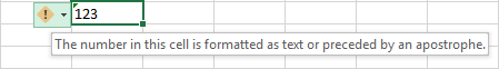

In some cases, an error indicator does not show up for numbers formatted as text. But there are other visual indicators of text-numbers:

In the image below, you can see the text representations of numbers on the right and actual numbers on the left: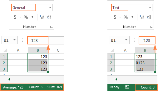

How to convert text to number in Excel

There are a handful of different ways to change text to number of Excel. Below we will cover them all beginning with the fastest and easiest ones. If the easy techniques don’t work for you, please don’t get disheartened. There is no challenge that cannot be overcome. You will just have to try other ways.

Convert to number in Excel with error checking

If your cells display an error indicator (green triangle in the top left corner), converting text strings to numbers is a two-click thing:

1. Select all the cells containing numbers formatted as text.
2. Click the warning sign and select Convert to Number.

Done!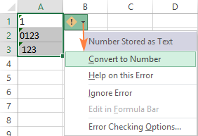

Convert text into number by changing the cell format

Another quick way to convert numerical values formatted as text to numbers is this:

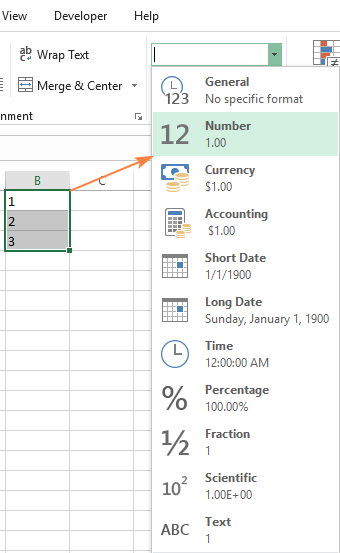
1. Select the cells with text-formatted numbers.
2. On the Home tab, in the Number group, choose General or Number from the Number Format drop-down list.

Change text to number with Paste Special

Compared to the previous techniques, this method of converting text to number requires a few more steps, but works almost 100% of time.

To fix numbers formatted as text with Paste Special, here’s what you do:

1. Select the text-number cells and set their format to General as explained above.
2. Copy a blank cell. For this, either select a cell and press Ctrl + C or right-click and choose Copy from the context menu.
3. Select the cells you want to convert to numbers, right-click, and then click Paste Special. Alternatively, press the Ctrl + Alt + V shortcut.
4. In the Paste Special dialog box, select Values in the Paste section and Add in the Operation section.
5. Click OK.

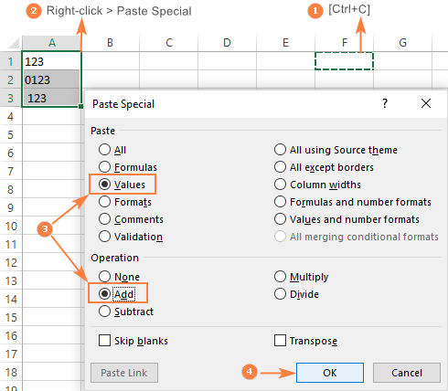
If done correctly, your values will change the default alignment from left to right, meaning Excel now perceives them as numbers.

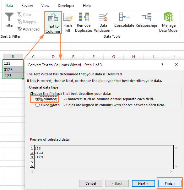
Convert string to number with Text to Columns

It is another formula-free way to convert text to number in Excel. When used for other purposes, for example to split cells, the Text to Columns wizard is a multi-step process. To perform the text to number conversion, you click the Finish button in the very first step 🙂

1. Select the cells you’d like to convert to numbers, and make sure their format is set to General.
2. Switch to the Data tab, Data Tools group, and click the Text to Columns button.
3. In step 1 of the Convert Text to Columns Wizard, select Delimited under Original data type, and click Finish.

That’s all there is to it!

Convert text to number with a formula

So far, we have discussed the built-in features that can be used to change text to number in Excel. In many situations, a conversion can be done even faster by using a formula.

Formula 1. Convert string to number in Excel

Microsoft Excel has a special function to convert a string to number — the VALUE function. The function accepts both a text string enclosed in quotation marks and a reference to a cell containing the text to be converted.

The VALUE function can even recognize a number surrounded by some «extra» characters — it’s what none of the previous methods can do.

For example, a VALUE formula recognizes a number typed with a currency symbol and a thousand separator:

To convert a column of text values, you enter the formula in the first cell, and drag the fill handle to copy the formula down the column: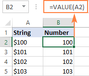

Formula 2. Convert string to date

Apart from text-numbers, the VALUE function can also convert dates represented by text strings.

Where A2 contains a text-date.

By default, a VALUE formula returns a serial number representing the date in the internal Excel system. For the result to appear as an actual date, you just have to apply the Date format to the formula cell.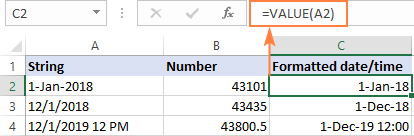

The same result can be achieved by using the DATEVALUE function:

Formula 3. Extract number from string

The VALUE function also comes in handy when you extract a number from a text string by using one of the Text functions such as LEFT, RIGHT and MID.

For example, to get the last 3 characters from a text string in A2 and return the result as a number, use this formula:

The screenshot below shows our convert text to number formula in action: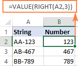

If you don’t wrap the RIGHT function into VALUE, the result will be returned as text, more precisely a numeric string, which makes any calculations with the extracted values impossible.

Change Excel string to number with mathematic operations

One more easy way to convert a text value to number in Excel is to perform a simple arithmetic operation that does not actually change the original value. What can that be? For example, adding a zero, multiplying or dividing by 1.

If the original values are formatted as text, Excel may automatically apply the Text format to the results too. You may notice that by the left-aligned numbers in the formula cells. To fix this, be sure to set the General format for the formula cells.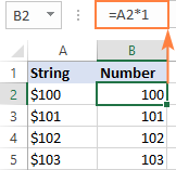

That’s how you convert text to number in Excel with formulas and built-in features. I thank you for reading and hope to see you on our blog next week!

How to convert text to number in Excel

The tutorial shows many different ways to turn a string into a number in Excel: Convert to Number error checking option, formulas, mathematic operations, Paste Special, and more.

Sometimes values in your Excel worksheets look like numbers, but they don’t add up, don’t multiply and produce errors in formulas. A common reason for this is numbers formatted as text. In many cases Microsoft Excel is smart enough to convert numerical strings imported from other programs to numbers automatically. But sometimes numbers are left formatted as text causing multiple issues in your spreadsheets. This tutorial will teach you how to convert strings to «true» numbers.

How to identify numbers formatted as text in Excel

Excel has an inbuilt error checking feature that alerts you about possible problems with cell values. This appears as a small green triangle in the top left corner of a cell. Selecting a cell with an error indicator displays a caution sign with the yellow exclamation point (please see the screenshot below). Put the mouse pointer over the sign, and Excel will inform you about the potential issue: The number in this cell is formatted as text or preceded by an apostrophe.

In some cases, an error indicator does not show up for numbers formatted as text. But there are other visual indicators of text-numbers:

In the image below, you can see the text representations of numbers on the right and actual numbers on the left:

How to convert text to number in Excel

There are a handful of different ways to change text to number of Excel. Below we will cover them all beginning with the fastest and easiest ones. If the easy techniques don’t work for you, please don’t get disheartened. There is no challenge that cannot be overcome. You will just have to try other ways.

Convert to number in Excel with error checking

If your cells display an error indicator (green triangle in the top left corner), converting text strings to numbers is a two-click thing:

1. Select all the cells containing numbers formatted as text.
2. Click the warning sign and select Convert to Number.

Done!

Convert text into number by changing the cell format

Another quick way to convert numerical values formatted as text to numbers is this:

1. Select the cells with text-formatted numbers.
2. On the Home tab, in the Number group, choose General or Number from the Number Format drop-down list.

Change text to number with Paste Special

Compared to the previous techniques, this method of converting text to number requires a few more steps, but works almost 100% of time.

To fix numbers formatted as text with Paste Special, here’s what you do:

1. Select the text-number cells and set their format to General as explained above.
2. Copy a blank cell. For this, either select a cell and press Ctrl + C or right-click and choose Copy from the context menu.
3. Select the cells you want to convert to numbers, right-click, and then click Paste Special. Alternatively, press the Ctrl + Alt + V shortcut.
4. In the Paste Special dialog box, select Values in the Paste section and Add in the Operation section.
5. Click OK.

If done correctly, your values will change the default alignment from left to right, meaning Excel now perceives them as numbers.

Convert string to number with Text to Columns

It is another formula-free way to convert text to number in Excel. When used for other purposes, for example to split cells, the Text to Columns wizard is a multi-step process. To perform the text to number conversion, you click the Finish button in the very first step 🙂

1. Select the cells you’d like to convert to numbers, and make sure their format is set to General.
2. Switch to the Data tab, Data Tools group, and click the Text to Columns button.
3. In step 1 of the Convert Text to Columns Wizard, select Delimited under Original data type, and click Finish.

That’s all there is to it!

Convert text to number with a formula

So far, we have discussed the built-in features that can be used to change text to number in Excel. In many situations, a conversion can be done even faster by using a formula.

Formula 1. Convert string to number in Excel

Microsoft Excel has a special function to convert a string to number — the VALUE function. The function accepts both a text string enclosed in quotation marks and a reference to a cell containing the text to be converted.

The VALUE function can even recognize a number surrounded by some «extra» characters — it’s what none of the previous methods can do.

For example, a VALUE formula recognizes a number typed with a currency symbol and a thousand separator:

To convert a column of text values, you enter the formula in the first cell, and drag the fill handle to copy the formula down the column:

Formula 2. Convert string to date

Apart from text-numbers, the VALUE function can also convert dates represented by text strings.

Where A2 contains a text-date.

By default, a VALUE formula returns a serial number representing the date in the internal Excel system. For the result to appear as an actual date, you just have to apply the Date format to the formula cell.

The same result can be achieved by using the DATEVALUE function:

Formula 3. Extract number from string

The VALUE function also comes in handy when you extract a number from a text string by using one of the Text functions such as LEFT, RIGHT and MID.

For example, to get the last 3 characters from a text string in A2 and return the result as a number, use this formula:

The screenshot below shows our convert text to number formula in action:

If you don’t wrap the RIGHT function into VALUE, the result will be returned as text, more precisely a numeric string, which makes any calculations with the extracted values impossible.

Change Excel string to number with mathematic operations

One more easy way to convert a text value to number in Excel is to perform a simple arithmetic operation that does not actually change the original value. What can that be? For example, adding a zero, multiplying or dividing by 1.

If the original values are formatted as text, Excel may automatically apply the Text format to the results too. You may notice that by the left-aligned numbers in the formula cells. To fix this, be sure to set the General format for the formula cells.

That’s how you convert text to number in Excel with formulas and built-in features. I thank you for reading and hope to see you on our blog next week!